 Australia
 International


 Blogs
Blogs Glossary
 Templates
 Videos
 Paperback Literature
Key Words
Progress. Position. Forecast. Earned value. Change. Linear regression. S-curve. Schedule.
Abstract
Current methods for assessing activity progress, calculating project position and forecasting project completion (including the use of earned value analysis) are examined in this paper. The disadvantages of current forecasting methods are discussed with special reference to single data point extrapolation and the difficulty for non-specialists in analysing s-curves. A different method of forecasting project completion using simple linear regression and time series analysis is proposed which has real practical applications for project managers and allows them to easily and rapidly produce position and forecast data in a format that is understood by layman and specialist.
Introduction
The UK Construction Industry does not have a good record for completing projects on time. Constructing Excellence’s data from its 2012 report (the latest available) shows that the actual out-turn time taken for the construction phase of projects compared with the length of time agreed at the start of that phase dropped sharply in 2012, with only 42% of projects delivered on time or better, compared with 60% the year before. Whilst this is the first time since 2000 that the KPI was below 50% the data shows that, on average, less than 40% of projects finish on time, Figure 1.
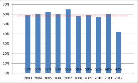
Figure 1. Predictability Time - Construction
The production of a project schedule is the first step in project control. In some cases, particularly on undemanding and straightforward projects, this initial planning and programming is sufficient and the project manager will be able to determine the status of the project without rigorous examination. More often schedules are required to assist with the active management of time by regular monitoring, examination and modification. Active management of time comprises three steps; Progress, Position, and Prediction, these are all relative to a point in time when the measurements or calculation are made; ‘time now’. Without accurate measurement of progress it is not possible to establish the position of the project and without knowing the current status of the project, predictions about the completion of the project are likely to be little more than guesswork. Without knowing when the project is likely to be complete it is impossible to determine what action must be taken to bring in the project on time.
Current Techniques
Progress – how much has been done
This is reasonably straightforward and usually involves assessment or calculation of the percentage of work completed on individual schedule activities. Progress can also be attributed to the project as a whole but unless the project is relatively simple a single measure of how much of the project is complete is somewhat superficial.
Position – what is the current status
Position is usually stated as time ahead, on schedule or time behind and relates to an individual activity or the project as a whole is a comparison of where the activity, or project, is compared to where it was planned to be.
For a single activity, assessment or calculation of position is also relatively straightforward. To calculate activity position:
if S TN F, then if (% < 100, P = S + (D x %) – TN, else P = 0), else
if S TN F, then P = S + (D x %) – TN, else
if S TN, then if (% > 0, P = S + (D x %) – TN, else P = 0)
Where: P is the activity position,
S is the planned start of the activity,
F is the planned finish of the activity,
TN is time now,
D is the planned duration of the activity, and
% is the percentage complete of the activity at time now.
However, for a single activity, position is more readily demonstrated graphically using the bar chart ‘drop line’ method (see figure 2).
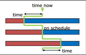
Figure 2. Drop line activity progress and position
Determining the project position (or project status) accurately is more difficult. Many project managers will use their skill, judgement and experience to assess the project position. However, such visceral and subjective techniques are open to suggestion of bias and manipulation for commercial or other ends.
A number of objective techniques have been developed:
- Averaging. This method averages the position of all the activities that are ahead or behind schedule. Although simple and apparently reasonable this method is mathematically unsound.
- Planned Progress Monitoring (PPM). This method compares the planned work content (based on activity duration) with that achieved. This method does not depend on the schedule being a critical path network and is predominately the underlying method adopted to ‘roll up’ progress in summary and expanded type bars of project management software.
- Critical Path Methods. When the progressed project is rescheduled with the variance in the end date of the project can be interpreted as the project position. This method depends on a fully linked and logical network.
- Earned Value Analysis (EVA). The parameter SV (scheduled variance) is a measure of the current status of the project. This is similar to standard cash flow analysis; income -v- expenditure or cash weighted PPM.
Prediction – when will the project end
Predicting is the estimation or forecasting of some future event or condition of the project as a result of the study and analysis of available data on the basis of observation, experience or scientific reason. Generally this will relate to a project milestone and particularly a forecast of when the project will be complete.
By its nature the prediction of future events with any degree of accuracy is difficult. Project managers tend to rely on their experience and analysis based upon the current position of the project and with the assistance of the project schedule will envisage, or more formally reassess, the schedule for the remaining work. If the reason for delay in the schedule was merely unrealistic durations and sequences then updating and amending the schedule to predict the completion date may be viable. Unfortunately the time taken to complete activities generally conforms to Parkinson’s Law and the Student Syndrome so, unless the underlying causes of delay are confronted, there is inherent risk of overrun of the reassessed schedule too.
The result of analysing a critical path network taking into account current progress is often erroneously referred to as a forecast of completion. For instance, where the project is in delay the rescheduled end date of the project would be delayed, this will only be a forecast of the completion date if the uncompleted remaining work were to be carried out in accordance with the schedule. It is more likely that if past work was not carried out in accordance with the schedule then, unless something changes, nor would future work. As stated previously the result of rescheduling a network taking account of current progress is a measure of the project position.
EVA attempts to formalise the forecasting of completion of projects using the parameter EAC (Estimate at Completion). The unnecessarily complex acronyms render the technique virtually unusable for all but the ardent enthusiast. In relation to time alone the technique can be simplified using the rate of progress to date and the time outstanding on the original schedule; for example, see Figure 3.
Planned completion date = 22.0 (BACt)
Time now = 12.0 (BCWSt)
Current position = 10.0 (BCWPt)
Rate of Progress = 10.0 / 12.0 = 0.83 (SPI)
Time not yet completed=22.0 – 10.00=12.0
Forecast time to complete = 12.0 / 0.83 = 14.5 (ETCt)
Forecast completion date = 12.0 + 14.5 = 26.5 (EACt)
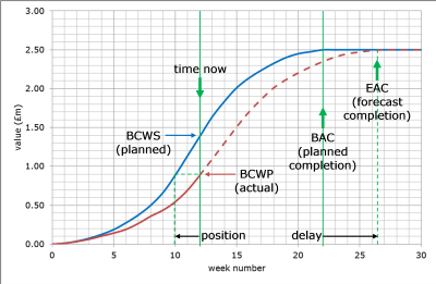
Figure 3. Forecast completion using Earned Value Analysis
Whilst the estimated completion date can be calculated, plotting of the remaining forecast to completion curve is problematic, but without it, it is difficult to envisage the remaining progress of the project and to determine if future work is proceeding to the forecast plan. In his booklet ‘EVA in the UK’, Steve Wake says:
The estimates to complete can be plotted (or hand-drawn by “experienced professionals”). …
The prediction of potential EACs (Estimates at Completion) has become increasingly accurate by using performance statistics from similar projects. These statistics become templates that are overlaid onto the existing cost curves of a project and provide an independent and objective estimate of the final cost and completion date. Something that everyone is interested in.
Blythe and Kaka take a different view and appear to suggest that advanced mathematical modelling is required (or at least beyond the capabilities of most project managers) and that the accuracy of the models is questionable:
There have been many attempts in the past to develop cash flow forecasting models. They were mainly part of more comprehensive models aimed at assisting contractors or clients forecast their cash flow on an individual project level or on a company level. The majority of these models were based on the idea of developing standard S-curves to represent the running value or cost of different types of construction projects. Typically this was achieved by collecting data relating to the monthly valuations and the projects’ general characteristics. These projects would then be classified and distributed into groups and average S-curves would then be fitted on the individual groups. Several mathematical models were used to fit the S-curves (e.g. alpha-beta cubic equation, Weibull function, DHSS model etc.). These models could be used, given that the total value and duration of the projects to be constructed are known, to forecast the cumulative monthly (or at any other time interval), value/cost of that project. The accuracy of these previous models is in question.
Using PPM similar shaped graphs to EVA’s BCWS and ACWP for planned progress and actual/as-built progress are generated. Whilst PPM is a useful method for determining the position of a project the s-curves that are typically produced are not easy for most practitioners to assimilate and to use for forecasting, see Figure 4.
Extrapolating the rate of progress, planned compared to actual at ‘time now’ can be used to predict the project completion date without the need for considering EVA or PPM. The only data require is the original project duration (D), the project position (P) and the ‘time now’ date (TN). The forecast completion date is:
Completion = D x TN / P
Using the previous example:
= 22 x 12 / 10 = 26.4
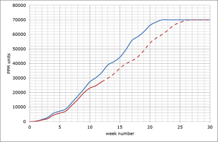
Figure 4. PPM - planned, actual and forecast curves
The Proposed Method – Simple Linear Regression
Statistical analysis of project data has, up to recently, been the preserve of the financial analysts, be they corporate accountants or project accountants. The data produced, when graphed, tends to resemble an s-curve. As described previously, in connection to EVA, it is not easy to estimate the path of a partially completed curve. It is possible, theoretically at least, to assign a mathematical formula to most curves but these can be extremely complicated (at least for the layman) and there is no certainty as to the shape, and hence formula, of that a predicted curve will, or should take.
The data for the graph at Figure 3 was based on SPI of 0.8 and further randomized on a monthly basis between 80% and 120% to model variances in progress. The graph at Figure 5 illustrates the difference between the forecast data (from Figure 3) and the modelled ‘actual’ data. The forecast completion is 27.6 months which is very close to 27.5 months that would be expected for a 22 month project (22/0.8). Whilst this apparent accuracy is as much to do with the coincidence randomness of the data it illustrates the primary flaw in SPI type forecasts that they use a single data point as the basis for extrapolation rather than a longer term trend.
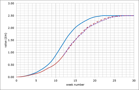
Figure 5. EVA - forecast and actual
To overcome this weakness and the limitations of projecting unsystematic curves the method described below is based upon simple linear regression and time series analysis. Whilst the components of the method are not novel the author is not aware of it being used to forecast project completion, particularly at least in the UK construction and engineering industry.
The planned model
The position of a project is usually stated as being ahead, on schedule or behind but it can also be stated as the number of schedule weeks achieved. For instance, a project at week 20 which is 2.5 weeks behind schedule can be said to have achieved week 17.5, similarly a project at week 20 that is 2.5 weeks ahead of schedule can be said to have achieved week 22.5. The importance of the proposed method is recognising that for all projects there is a simple straight-line relationship between the planned position of a project and project time such that, for instance, at week 20 the project is planned to have achieved week 20. The planned position line for all projects will be a ’45 degree’ line which straightens at the project completion date; see Figure 6. In terms of EVA the planned line is similar to the BCWS curve.
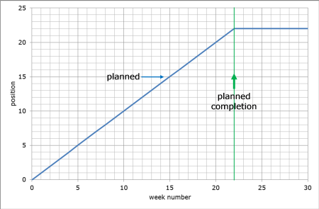
Figure 6. The actual/as-built model
The data for the actual/as-built model (BCWP in EVA parlance) is generated by calculating the project position by whatever method is appropriate as outlined above. It is not recommended that different methods of determining the project position are used for each period but it may be good practice to generate multiple datasets based on different methods of calculation which then may give a range of estimates of project position.
The actual/as-built position data can then be plotted against the planned data; see Figure 7. As the planned model is based on a straight line it is easier to appreciate the deviation of the actual position compared to the planned position.
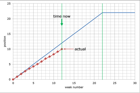
Figure 7. The actual/as-built model
The forecast model
The forecast of completion is made on the premise that, if nothing changes, if progress carries on in the future as it has in the past, the project completion date will be thus. Previous forecast models have used a single data point; the last measured project position. However trends are not absolute and there is likely to be some waxing and waning, positive and negative deviations from the general trend. Using the last measured progress position may exaggerate or understate the general trend.
As the planned position is based on a linear model it is acceptable to consider that the actual model, unless it is subject to wild fluctuations due to specific delaying events, will also follow a linear trend and hence forecast can be made using simple linear regression which will take account of all the past progress not just the last project position.
Figure 8 shows the simple linear regression line plotted for the actual project positions. The linear equation enables the trend line to be extended to the completion position (month 22) and for the date to be calculated, in this case 26.62 months.
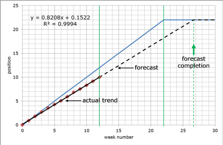
Figure 8. The forecast model
The position trends are easier to assimilate as straight lines and progress and trends, should future performance match past performance, can be readily seen as can changes in progress required if the project is to not lose any further time or to be completed on time, see Figure 9. It is submitted that such trends are not readily accessible using s-curves.
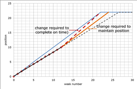
Figure 9. Change required
Most emphasis in this paper has been on projects that are behind schedule. Figure 10 shows typical regression plots for projects that are on schedule and for projects that are ahead of schedule.
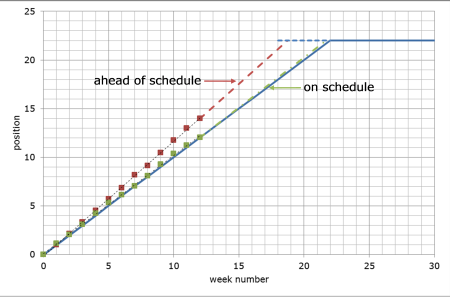
Figure 10. Ahead and on schedule
Conclusion
Forecasts of completion dates are almost always wrong. Forecasting completion of projects is not about estimating when a project will be complete but more about when it will be complete if progress continues in the future at the same rate that was achieved in the past. Only by knowing what the potential overrun (usually) will be if nothing changes can the project manager determine what needs to be done to bring the project back on schedule. The reason forecasts are wrong is that, hopefully, project managers will have taken steps, with the knowledge of the effects of doing nothing, and have pulled the project around.
Current methods of forecasting completion mostly depend on extrapolating the last known project position to forecast project completion. Earned Value methods also use a single position measure but depend on s-curves to illustrate the work flow. S-curves are difficult to assimilate and difficult to mathematically predict.
The proposed method depends on simple linear regression taking account of all the position data and presenting it in simple straight-line graphs that are more readily understood by non-specialists. Trends are easier to understand and the amount of action to bring the project back on schedule is straightforward to see.
Like all current methods of forecasting, including earned value methods, specific and exceptional delaying events can skew the forecast. Progress trends tend to be influenced by leadership, management, resources, experience and strategy decisions.
Acknowledgements
Anneka Wilson, Driver Group’s Group Marketing Executive has been constant with her help and encouragement even though, like most planners, I have always been behind schedule.
My colleagues at Driver Group; Stephen Lowsley, Keith Strutt, David Wileman, Philip Allington and Janus Botha have provided technical critique of my paper – any errors, however, remain mine.
Dr Chris Chatfield of the Department of Mathematical Sciences at the University of Bath and author of ‘The Analysis of Time Series: An Introduction, Sixth Edition’, kindly took time to reply to my emails and responded to my very basic time series questions.
Whilst every effort has been made to ensure the accuracy of the information supplied herein, Driver Group plc, its subsidiaries and the author cannot be held responsible for any errors or omissions. Unless otherwise indicated, opinions expressed herein are those of the author and do not necessarily represent the views of Driver Group plc and/or its subsidiaries.
The author warrants that he is the copyright owner and that all sources are acknowledged and referenced and that as far as it is possible to ascertain this work does not infringe any existing copyrights.
All rights reserved. No part of this document may be reproduced or transmitted in any form or by any means, electronic, mechanical, photocopying, recording, or otherwise, without prior written permission the author or Driver Group plc.


