To many managers in the construction industry value is overshadowed by cost. By not seeing the value that planning and scheduling can bring to a project, 98% of the project budget may be placed at risk in order to save a few dollars of the overhead budget. I categorize attitudes toward scheduling among those that consider scheduling a necessary project function as either ‘reactive’ or ‘proactive’. In addition, there is still a considerable part of the industry that does not schedule at all; we might say they have an ‘inactive’attitude to scheduling.

The difference between the proactive and reactive approach

The difference between the proactive and reactive approach is defined by the goal of the scheduling efforts. Reactive scheduling starts with a haphazard approach to the planning process and continues when the ongoing scheduling efforts are spent trying to keep up with happenings in the field, and making adjustments when field operations deviate from the scheduled plan. In this case the schedule may be built with good intentions, but the reality is that the project drives the schedule.

Proactive scheduling requires a coordinated effort of the project management staff to actually plan the work for the project and then utilize the scheduled plan in performing and overseeing the work in the field. Updates are performed to measure how the plan is going and to make necessary adjustments. The process of planning and scheduling is never complete until the project is done. In other words, the plan and schedule drives the project.

The Absurdity of Reactive Scheduling

I will never forget my first job as a professional scheduler. My contractor client informed me that my services were required to appease an ‘overzealous’ owner and were not necessary for success of the project. My services were merely a ‘necessary evil’. I proceeded to study the project documents and prepared the contractor’s schedule for submittal. The schedule clearly delineated how the project was to be built and was readily approved by the owner. My client received a long-awaited first payment on the project and I enjoyed hero status for a day.

However, the contractor’s project management team proceeded almost immediately to deviate from the schedule that I had spent so much effort to prepare. To my knowledge, no one on the contractor’s project management team ever put together a comprehensive plan for completing the project in a timely and efficient manner. The contract targeted completion date was a ‘hope for’ goal with no basis for the assumed accomplishment.

Since they had never really looked at my schedule, nor did they care to start, my task became increasingly an exercise in keeping up with what they were doing, and adjusting the schedule to show how their plan was deviating from mine. I also found myself trying to guess at what they might do in the future and make the appropriate adjustments in ‘my’ schedule. As the project slipped I would arbitrarily change relationships or durations to continue showing the project completion within the contract limits, which kept the cash flow coming from the owner. In no way did the schedule have any influence on the work performed. As the scheduler, I spent the majority of my effort trying to make the schedule match what was happening in the field,the project drove the schedule.

Schedule as a tool for planning the project

On the other side of the world, the owner reviewing my schedule never really looked at it as a tool for planning the project either. The only person who even looked at it on behalf of the owner was their expert scheduler, whose main objective was to make sure the schedule met the technical requirements of the contract specifications. The extent of the review was purely technical in nature. Did the numbers balance? Were the milestone dates aligned with the contract? Was the format of the schedule correct? The review and approval processes never included a review of whether or not the schedule was a valid plan or even whose plan it was. The only issue that seemed to matter was whether or not the document showed that the projected dates were being met.

No one ever mentioned to me that the contractor was not following their (my) plan. I don’t believe anyone ever paid enough attention to it to really notice. The people who really knew how the project would have to be constructed did not care to look at the technical data generated by a computer that they saw as a threat to the world as they knew it. The schedule was simply a required exercise someone passed down from a lofty legal bureaucracy on a planet far, far, away. On the other hand, the two scheduling experts (including myself) were too busy trying to impress each other with our own schedule geek techno jargon, and philosophical homilies regarding schedules and like things pertaining to it, to think about coordinating our efforts with the less technical project management staff who oversaw the actual construction. Even from the owner’s side, the project drove the schedule.

The Benefits of Proactive Scheduling

On many projects over the years my schedules were completely separate from the construction process. Contractors submitted them but didn’t use them. Owners were often contractually separated from the process and had minimal enforcement capability in how a schedule was managed. Times haven’t changed much. But there is hope. I have seen it work. Planning and scheduling can be used in a proactive way to make a project move faster, more efficiently, and with much less management headache. There are four main aspects of proactive construction scheduling, if implemented, these will positively transform the project at all levels.

Coordination and Collaboration

Though intertwined in practice, it is helpful to consider these separately. Coordination is bringing the various project participants into the planning process, securing their input and getting everyone to sign on to the project plan. The participants naturally include those actually building the project, including project managers, superintendents, subcontractors and yes, even the owner and their representatives. I often hear the first months of the project referred to as the ‘honeymoonv phase. If agreements are going to be made and cooperative measures are to be coordinated for the project, this is the period most beneficial to meet those objectives. By coordinating through the planning and scheduling process, each aspect and phase of the project can be addressed and reviewed by the parties.

Collaboration is the ongoing use of the schedule throughout the project as a communication tool to identify, address, and resolve project issues. To accomplish this, the contractorvs project management must be committed to communication and a level of openness with the various project participants, including the owner. Owners are usually more open to the idea but have a difficult time enforcing collaboration.

Consistent Tracking and Analysis

Consistent tracking and analysis of progress requires a level of scheduling discipline that is often lacking, but where it exists the rewards are substantial. For example, it is much easier to prepare a lookahead schedule with a handwritten chart or spreadsheet application than it is to update a working CPM schedule. Excuses such as vThe established schedule does not have the detail I need, or I only update the schedule for the submittal process, or ‘My schedule doesn’t match what I am doing’ are common. There is a simple response to such excuses: Adjust your schedule to reflect your plan so that you can use it to monitor your progress on a weekly or bi-weekly basis. Using this proactive approach in a project meeting may meet resistance because of the accountability involved.

The project accountability is a result of looking at what someone said they would do last week compared to what they are saying this week. Over time, however, such accountability serves to bring more consistent project planning and projections to the project. This level of project management tracking will also keep stakeholders aware of the project’s current critical path, which spreadsheet charts cannot do. One of the most important features of this proactive scheduling approach is the early identification of issues. Of course, early identification of issues promotes early resolution of issues, which is valuable in every project scenario.

Effective Project Reporting

Effective project reporting keeps senior management, the key decision makers and problem solvers, in the loop. Many project issues get out of control before senior management, or those with the most experience in resolving issues, ever get involved. This results from delays in identifying and communicating issues. A carefully monitored project plan and schedule will identify most issues as, or even before, they surface. An effective reporting procedure will keep executives in the loop to proactively resolves the issues before they become serious or get out of control. Risk Management and Early Resolution of Conflicts.

Proactive Construction Scheduling and Risk management

Risk management and early resolution of conflicts may be catchy industry buzz-phrases, but they are very important. This aspect of proactive construction scheduling depends on the implementation of the previous three proactive scheduling techniques. Without collaborative coordination, consistent tracking and analysis, and effective reporting, issues will often not be identified early enough for a quick resolution, and even when they are, the lack of a healthy cooperative atmosphere may impede that resolution. Part of updating the schedule regularly and proactively includes incorporating impacts immediately into the schedule to demonstrate their effects on the progress, and ultimately the completion of the project. This sometimes meets resistance. I have been requested not to put an impact into the schedule until the change or delay is approved. My response to this is simply, “Do you want the current project schedule, that we all are trying to work from, to be accurate or inaccurate?” If you want it to be accurate then what is going on in the field should be reflected in the schedule. I have yet to have someone tell me, “I would rather the construction schedule be inaccurate.” By incorporating issues into the schedule immediately it is much easier to see the impact and come to an early resolution.

Proactive Scheduling Pays

Ultimately, there is a cost factor to the proactive approach. It takes commitment from the involved parties and often it takes more management budget, especially if an experienced scheduler is brought in to assist in the process. However, the benefits from a successful implementation of the proactive approach usually far outweigh the costs associated with it. Managing the critical path effectively nearly always saves time on the project. Given the daily overhead costs of a project multiplied by the number of days saved by good planning and execution, this also saves money. Furthermore, regular planning and coordination brings a positive partnering atmosphere to the project. Reviewing a schedule is a great forum for structured discussion of every aspect of the project, since a good, proactive schedule will include every aspect. Finally, proactive scheduling is very effective in early resolution of disputes, maximizing recovery of cost impacts as well reducing the cost of prosecuting claims.

The role of CPM scheduling in the construction industry has increased significantly over the past couple decades. One reason for this is economic. Owners have become more demanding in their scheduling specifications in order to better monitor the project and meet funding requirements and budget projections. And tight competition and narrow profit margins have forced contractors to maximize efficiency through careful planning, scheduling, and coordination.

A second reason is liability. From claims preparation and dispute resolution to legal evidence in a trial, a well-designed and maintained CPM schedule can make or break the chances of recovering damages. Most fundamentally, however, a well-designed and maintained CPM schedule is just good project management practice—it lays out the road map that tells you how to get from point A to point B, from project start to project completion.

CPM Scheduling – The Project Road Map

Growing up in my family meant road-trip vacations every summer. And, of course, we asked all the typical questions children ask after sitting for hours in a back seat. The “How many more miles?” and “When are we going to get there?” questions were most often responded to with a map highlighted along the shortest path of travel (the “critical path”), and we were encouraged to figure out the answers ourselves. We learned that we could use the red numbers along the highway to measure progress and project our arrival time (duration). We could measure our average speed by counting the miles traveled divided by the hours on the road (production). Taking our average speed we could calculate our arrival time based on remaining miles (projections). What’s more, if my father made a wrong turn or we experienced mechanical difficulties, all we needed was the map to determine where we were when we went off course, how long we were off, and when we were safely back on the right path. From there we could measure the impact of the mishap.

These maps were great management tools. Not only did my parents use them to plan and make projections for the trip, they also were great for back seat management. The longer we went without getting the answers we needed the greater the noise level from the back seat. My parents learned early that an easy-to-read, clearly highlighted map kept us busy for hours and proved to be a good exercise in noise reduction and dispute management.

In any undertaking it is important to know where you are going, how you will get there, and what resources will be required to successfully achieve the goal. It is no different with any construction project. A successful project roadmap (a well-maintained construction plan) is an essential management tool for many of the same reasons that my parents learned in our vacation experiences.

A well thought-out plan and schedule will help in planning and allocating the five key resources on the project: time, money, personnel, equipment, and material. With that plan in place you only need to know three things to measure the impact of most delays: where you were on the critical path at the time of impact, how long you were off of the critical path, and when did you returned to full production on the critical activities. Finally, the well-prepared, easy-to-read plan is great for communication and noise management.

Create a New Project in Powerproject

In this video you will learn how to start a new Project in Elecosoft Powerproject, from an experienced construction scheduling consultant. Want the Training Manual?

Get the training manual for this series, as well as other great free resources for Powerproject, including a free Scheduling Template and more. To download visit our Powerproject Resources Page.

You must have a media player on your computer that can play video embedded in webpages, such as Quicktime

Abstract – With the variety of Delay Analysis Techniques available to schedule reviewers and analysts, it is difficult to know and implement the most reliable and effective way of demonstrating an accurate impact calculation caused by delay. Contractual requirements for time extension requests using the common term, “Time Impact Analysis”, are increasingly appearing throughout the construction industry. The broad application of the term “Time Impact Analysis” can lead to significant variances in delay calculations. Several of the AACE International’s Recommended Practices (29R-03) are commonly labeled as “Time Impact Analysis”. While each methodology may have its appropriate implementation, certain methodologies can be combined to produce a more reliable and accurate result. In the following paragraphs the Fixed Perspective Windows Delay Analysis (“Analysis”) method will be presented, which incorporates the strengths of various retrospective methods, while minimizing, if not alleviating the weaknesses. The result is an analysis that, when prepared correctly, is simple to calculate and easy to defend.

With the variety of Delay Analysis Techniques available to schedule reviewers and analysts, it can be difficult to identify and implement the most reliable and effective way of demonstrating an accurate impact calculation caused by delay in retrospect. Each analysis method has strengths and weaknesses with a series of validation requirements, so proper application of the various methods is essential to a reliable conclusion. The “Time Impact Analysis” is the method recommended within the Society of Construction Law Delay and Disruption Protocol.

In this method time impact analysis preparation includes the insertion of a delay activity into the sequence of unimpacted activities in a schedule prior to the delay event. The analyst can then determine the impact of the delay by measuring the impact to the prior completion date. Many, if not most, contract specifications that address preparation of time impact analyses are specifying a method that generally aligns with the method outlined by the Society of Construction Law. This method is virtually identical to that outlined in the AACE’s 29R-03 MIP 3.7. In addition, this methodology is similar to that which is outlined in the AACE document for prospective TIA preparations, 52R-06, with the notable exception that actual dates of the delay be used, retrospectively.

As will be detailed in the enclosed analysis, these referenced methodologies can be easily manipulated to reach biased results.

However, as construction scheduling requirements and specifications have become more stringent over the last few decades, it is possible to minimize these manipulations. More projects require monthly updates, more project staff are involved in the scheduling process, and more stakeholders provide input into the scheduling process. With increased experience and participation schedules are increasingly more consistent and accurate. Contemporaneously prepared schedule information is available more often. Delay analysis methods that rely on and incorporate this available schedule data will be consistently more reliable and accurate.

In the following paragraphs the Fixed Perspective Windows Delay Analysis (“Analysis”) method will be presented, which incorporates the strengths of certain retrospective, observational and additive methods while minimizing, if not alleviating the weaknesses. The Analysis identifies delay including mitigation and acceleration quantities, identifies concurrency, and accounts for changes in the critical path. It is equally significant to note that the Analysis will demonstrate how to select which schedule to use for the analysis to minimize manipulation. The result is an analysis that, when prepared correctly, is relatively simple to calculate and, just as importantly, easy to defend.

Common Problems with Contract Specified Delay Analyses (MIP 3.6 and MIP 3.7)

The AACE document for prospective TIA preparations, 52R-06 [2], details a recommended protocol for preparing Time Impact Analyses using a forward-looking approach. However, most project owners are hesitant to grant time extensions until the full extent of the delay is known. In shorter delays this may not be as challenging. However, on longer delay events, where the anticipated delay duration is not known, a retrospective approach is usually preferred by owners. The enclosed methodology is useful when contract documents require the actual durations of the delay and not the “forward looking” analysis detailed in 52R-06. The analysis may be prepared during the project or after, but is retrospective in time and incorporates Method Implementation Protocol (MIP) 3.7 – Retrospective, Modelled, Additive, Multi-based analysis.

The AACE document for prospective TIA preparations, 52R-06 [2], details a recommended protocol for preparing Time Impact Analyses using a forward-looking approach. However, most project owners are hesitant to grant time extensions until the full extent of the delay is known. In shorter delays this may not be as challenging. However, on longer delay events, where the anticipated delay duration is not known, a retrospective approach is usually preferred by owners. The enclosed methodology is useful when contract documents require the actual duration's of the delay and not the "forward looking" analysis detailed in 52R-06. The analysis may be prepared during the project or after, but is retrospective in time and incorporates Method Implementation Protocol (MIP) 3.7 – Retrospective, Modelled, Additive, Multi-based analysis.

As an example, a contractor may submit a Request for Information ("RFI") early in a project for installation of light fixtures that are not scheduled to be installed until very late in the project. Since the fixtures are not scheduled for installation for several months into the future, the architect may not respond immediately to the RFI. In the meantime, additional unrelated delays push the scheduled fixtures installation even further into the future. As a result, the actual duration for the response to the Request for Information extends even longer. Eventually, the architect responds to the RFI with a change. The change delays the installation of the fixtures a few days impacting the completion of the project.

In this scenario, the contractor, may choose to submit a TIA, prepared in an early schedule with the planned future duration's (blindsight) around the time of the initial RFI submission. The TIA specification states that delays should be analyzed by inserting actual delay duration's (hindsight) into a schedule just prior to the delay. Using the older schedule and the actual duration of the RFI response, the analysis would appear to demonstrate the RFI was on the critical path its entire duration, ultimately impacting the end date. By not incorporating details included in subsequent updates during the alleged delay period, the analysis misrepresents the real impact of the RFI and change.

In the following chart, Delay Event 1, representing a hindsight as-built duration of a delay activity, is inserted into a copy of a contemporaneously updated schedule. This analysis seems to demonstrate that the Delay Event 1 impacted the critical path of the project.

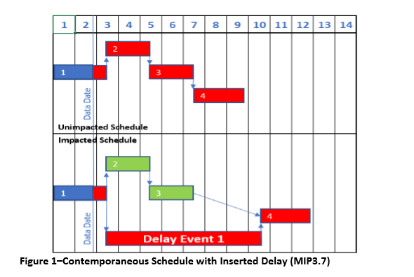
However, if the contemporaneous schedules are reviewed, the Delay Event 1 may have never been on the critical path until much later in the analysis period, once float was consumed. The following graphic illustrates a contemporaneous updated schedule with a data date in month 6 in which the Delay Event 1 is not driving the critical path. In many cases, the Delay Event 1 may not even be in the contemporaneous schedule since it is not driving an activity contemporaneously as of the data date.In this scenario, the Delay Event 1 may, or may not be a concurrent delay depending on available float and its management.

Another scenario is that the Delay Event 1 only becomes critical in a later contemporaneous update, once float is consumed. Following the completion of the Delay Event 2 impacted activities, Delay Event 1 becomes critical in the Month 10 schedule.

Using the previous examples, it is apparent that a delay analysis can be manipulated applying MIP 3.6 or 3.7 simply based on the application of terms detailed in the typical TIA specifications. This is why an Observational review of contemporaneous schedules during the delay period should be incorporated. The additive model of MIP3.7 may not include concurrent delays occurring during the delay event, or more significantly, it may not take into account changes in the critical path occurring during or prior to the delay event. In addition, TIA's are often prepared without consideration of contemporaneous updates within the delay period, which may impact the TIA's outcome. It is not uncommon for TIA's to be prepared that analyze delay events that never appear on the project’s contemporaneous updated schedule’s critical paths.

The questions remain, how can an analyst be reasonably certain when a delay impacted the critical path? How can the start of the actual delay period be reasonably identified? How can the end of the delay period be accurately be identified? How can the added or prolonged delay duration be quantified? And, how can an analysis determine if or when a particular delay was overtaken on the critical path by another delay? The following paragraphs detail an approach for preparing a single based or multi-based TIA (MIP 3.6 or 3.7), where each of these considerations are addressed and, as a result, the TIA is more reliable and more importantly, defendable. In summary, the Analysis addresses and corrects the common TIA specification approach of inserting delay events into a schedule prior to the delay event. “Prior to the delay event” is often manipulated and, based in the arguments below, should be adjusted to state, “Prior to the when the delay event became critical”.

How the Fixed Perspective Window Analysis Method fits into the AACE International’s RP for Forensic Scheduling

As stated in the previous section, the Analysis is a two-stepped process for analyzing delays that incorporates sections of the AACE International’s 29R-03 Recommended Practices. The Analysis is a retrospective approach that incorporates both the observational and modeled approach.

The first step includes the exercise of reviewing a Progress Period Window Looking Forward and Backward as part of the Observational model, Dynamic Logic Observation, and more specifically the Contemporaneous / As-Is and/or Contemporaneous / Split, MIP 3.3 or 3.4 [1]. This approach provides the analyst with an opportunity to review the project’s critical path, as memorialized during the project, before and after the delay event, and as documented in the submitted schedule updates. It is an accurate quantification of the delay event from start to finish, including the time frame of when the delay event became critical and when it was finished or when another event took over the critical path.

The analysis requires the project baseline schedule and periodic schedule updates that were prepared contemporaneously during the project, and whose network logic may differ to varying degrees from the baseline and from update to update [1]. It can be implemented using all periods or grouped periods as long as each individual period is reviewed to ensure a comprehensive analysis and to avoid utilization of subjectively selected data.

The second step in the Analysis incorporates the findings of the first step into the Modeled approach, specifically the Additive Modeling with the Single Base or Multi-Base, as defined in MIP 3.6 or 3.7, or the "TIA", in order to meet the common contractual requirements for measuring project delays.

Prerequisites for Preparation of the Fixed Perspective Windows Analysis

Prior to preparation of the Analysis a thorough review of the baseline and monthly updated schedules should be performed with sufficient and appropriate Source Validation Protocols as detailed in the AACE 29R-03 SVP 2.1 – 2.4. Although the AACE RP for Forensic Scheduling states that "Forensic Scheduling is a technical field associated with, but distinct from, planning and scheduling field", experience with planning and schedule is essential in order to avoid misapplication of the enclosed analysis. The analyzer “is assumed to have advanced, hands-on knowledge of all components of CPM analysis and a working experience in a contract claims environment involving delay issues”[1]. A hands on, in-the-field scheduling experience is also valuable.

Performing a Fixed Perspective Windows Analysis – Part 1

The Fixed Perspective Window Analysis in the enclosed Analysis is a detailed and multi-view analysis of a period, or window, of project time using the contemporaneous time frame schedule updates prepared during the course of the project. The analysis is multi-view in that it reviews the fixed window of time from two perspectives, before and after the window of time. The term fixed perspective addresses a common generalization about the windows analysis method where analysts define their own time periods, often subjectively and materially affecting the end results. The analysis is prepared one window at a time. It assumes the periodic schedule updates are reasonably accurate, and the Source Validation Protocols for baseline schedules and updates have been reviewed.

The Analysis is a two-step approach to preparing the traditional TIA that ensures an accurate and reliable result when calculating delay events. It incorporates the fixed approach of reviewing the contemporaneously prepared schedule updates without modification (MIP 3.3) and incorporating the results of that review into an additive model (MIP 3.7), required in a common TIA contract specification. The review requires that each of the Critical Path Method (CPM) schedules, prepared during the project, be used. The critical path activities are the primary activities analyzed with their associated changes and impacts.

The goal of the Analysis is to isolate only those delays that impacted the critical path and ultimately the completion of the project. Therefore, the Analysis does not attempt to analyze every delay event, but only the critical path delay events as they impacted completion once construction began. The Analysis includes both an as-built critical path analysis to accurately identify and analyze any changes or delays to the critical path, and project completion included in the submitted schedules (MIP3.3). It also includes a contemporaneous analysis of delays (MIP3.7) whereby the delay issues are inserted into the schedule update nearest to the actual start of the delay issues, in order to meet a TIA contract requirement. The methodology includes a detailed review of each project schedule update prepared during the project, analyzing the specific periods between the schedule updates as “progress period windows”. The review includes: 1) a review of the progress period window looking forward, using the schedule update prior to the progress period window; and 2) a review of the progress period window looking backward, using the schedule update at the end of the progress period window. This is illustrated in Figure 4.

The first step in preparing the Analysis incorporates a review of specific “windows” of time looking forward using a static model of the contemporary updates, an implementation of AACE International’s 29R-03, MIP 3.3. The Fixed Perspective Window Analysis Looking Forward includes a detailed analysis of each progress period (periods in between monthly updates), or a window analysis. First, the analyst should perform a detailed review of the critical path in the monthly update prior to the progress period window. Second, a progress verification is performed comparing the planned critical path activities to actual performance included in the subsequent updated schedule. Third, the monthly update critical path is compared to actualized performance in the subsequent update to verify whether the critical path had changed during the reported period. Finally, changes in sequence and/or duration's are reviewed to determine if the critical path changed during the period.In addition, changes in future planned activities are evaluated to determine schedule impacts, gains, or losses outside of the selected evaluation period in order to demonstrate how overall changes impacted the final completion date.

In addition to delay impacts, the Analysis identifies and quantifies efforts made through re-sequencing work activities, or reduced duration's that may have recovered time during the project, incorporating MIP 3.4[1]. The following paragraphs include a review of two windows from a sample project to demonstrate delay calculation using the Fixed Perspective Window Analysis.

The Forward-Looking Window Analysis for Period 1

Figure 5 includes a bar chart from a contemporaneous schedule (Schedule 1) compared to a subsequent schedule update with a data date one month later (Schedule 2). The Forward-Looking comparison is comparing changes that occurred to the critical path in the subsequent updated schedule. The spreadsheet area of the bar chart schedule includes three columns: the activity name, variance in start dates, and variance of finish dates. The comparison bars for Schedule 2 are shown below the Schedule 1 bars. The color of the bars indicates whether the activities are critical or not in both schedules. As an example, the top bars for the Phase 1 activities are red indicating that they are critical in the current schedule, while the comparison bars are black, indicating that, in the subsequent schedule, the activities are no longer critical. The first three activities in the “Phase 2” section were not critical, but in the subsequent schedule these activities have become part of the critical path. Notations are numbered and include in a Table 1 after the bar chart.

The following comments in Table 1 detail notations from Figure 5.

The Backward-Looking Window Analysis for Period 1

Figure 6 includes a bar chart from the contemporaneous schedule (Schedule 2) compared to a previous schedule update with a data date one month earlier (Schedule 1). This perspective is reviewing the same time frame as Figure 5, except comparing changes that occurred to the critical path in the previous updated schedule. The spreadsheet area of the bar chart schedule includes the same three columns: the activity name, variance in start dates, and variance of finish dates. The comparison bars for Schedule 1 (previous update) are shown below the Schedule 2 bars (subsequent update). Once again, the color of the bars indicates whether the activities are critical or not in both schedules.

As an example, the top bars for the Phase 1 activities are not red indicating that they are no longer critical in the current schedule, while the comparison bars are red, indicating that, in the previous schedule, the activities were critical. The first three activities in the “Phase 2” section were not critical, but in the subsequent schedule these activities have become part of the critical path. In this window of time between Schedule 1 and Schedule 2 the notations are identical and are detailed in the previous Table 1.

A summary of the events in the first window are detailed in Table 2. In summary, the delay event impacted the critical path 18 days. Considering the gain in production of the previous critical activity of 1 day, the net result to the schedule is a 17-day loss.

The Forward-Looking Window Analysis for Period 2

Period 2 is the subsequent month from the month analyzed in Period 1. Figure 7 includes a bar chart from the contemporaneous schedule (Schedule 2) compared to the subsequent schedule update with a data date one month later (Schedule 3). The Forward-Looking comparison is comparing changes that occurred to the critical path in the subsequent updated schedule. The spreadsheet area of the bar chart schedule includes the same three columns as the previous bar charts: the activity name, variance in start dates, and variance of finish dates. The comparison bars for Schedule 3 are shown below the Schedule 2 bars. The color of the bars indicates whether the activities are critical or not in both schedules.

As an example, the top bars for the Phase 2 activities are red indicating that they are critical in the current schedule, while the comparison bars are black, indicating that, in the subsequent schedule, the activities are no longer critical.

There is a gap between the activities, “Exc/Grade Detours” and “Pave Detours”. This is indicative of added activities in the subsequent schedule (or extended duration's if a filter is being used) causing a change in the critical path.

Notations are numbered and included in Table 3 following the bar chart.

The following comments in Table 3 detail notations from Figure 7. Identification of recovery/acceleration in the schedule comparisons coincide with the MIP 3.4 criteria.

The Backward-Looking Window Analysis for Period 2

Figure 8 includes a bar chart from the contemporaneous schedule (Schedule 3) compared to a previous schedule update with a data date one month earlier (Schedule 2). This perspective is reviewing the same time frame as Figure 7. The spreadsheet area of the bar chart schedule includes the same three columns: the activity name, variance in start dates, and variance of finish dates. The comparison bars for Schedule 2 (previous update) are shown below the Schedule 3 bars (subsequent update). Once again, the color of the bars indicates whether the activities are critical or not in both schedules. As an example, the top bars for the Phase 2 activities are not red, indicating that they are no longer critical in the current schedule. While the comparison bars are red, indicating that, in the previous schedule, the activities were critical. The first two activities in the “Phase 2” section were critical, but in the subsequent schedule these activities were no longer on the critical path. Notations from Figure 8 are included in Table 4. The comments are similar to the Forward-Looking comparison with added information from the later schedule, unavailable in the forward-looking schedule.

A summary of the events in the second window of time are detailed in Table 5 below. In summary, the Delay Event 1 impacted the critical path an additional 19 days. Another Delay Event (Delay Event 2 – Paving Mix Design Resolution), impacted the critical path an additional 10 days this period. Subsequent re-sequencing reduced the impacts by 10 day for a net loss of 19 days this period. With the 18 days lost in the previous period the net loss by Delay Event 1 is 36 days.

NOTE: There are two issues not in these conclusions: 1) Delay Event 2 overtook Delay Event 1 on the critical path 10 days prior to its planned completion date in Schedule 3. No conclusions were drawn regarding any of the overlap period that may have been a concurrent delay. 2) The gain resulting from resequencing may be contributed to either delay depending upon which party initiated the recovery/acceleration efforts.

Performing a Fixed Perspective Windows Analysis – Part 2

.Part 2 of the Analysis complies with the 29R-03 MIP 3.7 and 52R-06 Time Impact Analysis, if the reviewer is requiring a known completion of the delay period (retrospective). Part 1 identified the duration of the delay events and when the various delay events impacted the critical path. With this information, separate and often overlapping delays can be inserted into the appropriate schedule prior to the start of the delay’s impact to the critical path. In the above example Delay Event 1 impacted the critical path in Schedule 2. Therefore, the appropriate schedule in which to insert a delay activity representing Delay Event 1 (37 days) is in Schedule 1. Delay Event 2 impacted the critical path in Schedule 3. Therefore, the appropriate schedule for the MIP 3.7 analysis of Delay Event 2 is in Schedule 2.

The Advantages of the Fixed Perspective Window Analysis

The previous Analysis meets all of the Underlying Fundamentals and General Principals laid out in the AACE Recommended Practices for Forensic Scheduling,: 1) It uses CPM Calculations; 2) The concept of Data Date is an integral part of the Analysis; 3) network float is identified and accounted for; 4) Float is based on the appropriate schedule; 5) Sub-Network Float can also be evaluated when needed; 6) the calculation of impacts can be demonstrated in relation to the critical path; and, 7) all available schedules are considered. Preparing an analysis as described herein, where Impacts of potential causes of delay are evaluated within the context of the schedules in effect at the time when the impact or multiple impacts happen, increases the accuracy in quantification. In addition, the fixed time periods provide the best as-built of not only project dates and sequences, but an as-built view of the prospective critical path as contemporaneously prepared.

Conclusion

Guidelines for preparation of Time Impact Analyses prescribed in many contract specifications align with the MIP 3.7 methodology. The guidelines can be vague and easily manipulated. Therefore, a proper application of a Time Impact Analysis methodology is essential to reach a reliable conclusion. The enclosed method for measuring delays incorporates the strengths and minimizes the weaknesses of common delay analyses by combining an application of MIP 3.3 to MIP 3.7. The combination, as described in the previous paragraphs, will minimize errors and manipulations by identifying the appropriate schedule to use as a basis for the Time Impact Analysis and a reliable duration of the analyzed delay, while meeting the typical contract requirement for preparing a TIA.

Lets first understand what is QRA and Monte Carlo?

Quantitative Risk Analysis (QRA) is a forecasting technique used to predict project cost and/or schedule outcomes, and to estimate an appropriate level of contingency. The QRA seeks to develop realistic project schedules and estimates for a genuine prediction on how the project may result. In the past, project contingency has often been set by means of an uplift (E.g. 10% on cost/time). This approach is rudimentary, often provides no justification on why a certain uplift is applied, and may result in an entirely inadequate risk contingency.

There is generally a finite number of occasions on which a project can baseline schedules/budgets; we can maximise our chances of success by utilising Monte Carlo Analysis (MC).

Monte Carlo is a mathematical technique utilising random sampling, within specified distributions to calculate the probability of explicit outcomes. The underlying principal of the method is rooted in the law of averages, and the law of large numbers; creating a mathematical prediction of how the process may eventuate.

MC uses input duration ranges, as opposed to single point estimates for activity durations, to offset the inherent uncertainty in estimating. For a holistic coverage of possible cost/schedule outcomes, Risk Events (with a defined probability of occurrence, as well as an impact duration range) can be assigned to activities within the programme and contribute to the analysis (effectively extending the linked activity by the nominated impact duration value, on any iteration in which it appears). The Risk Analysis model is simulated hundreds, or thousands of times, and on each iteration a value is randomly selected from within the defined duration range for each activity. The most widely used, and easily understandable, range distribution is a triangular distribution (often referred to as a 3-point estimate and provided as a minimum, most likely, and maximum). The MC simulation is entirely random, plotting the outputs of each iteration as it works to create several useful insights. MC analysis undertaken on a project schedule takes cognisance of logic uncertainty and calendars, creating forward and backward pass calculations for each relationship in the plan, ultimately providing confidence intervals based on the range of start/finish dates for each milestone/activity.

Cumulative distribution graphs (S-curves) can be created to inform probability distributions (from which we can extrapolate confidence percentiles e.g. P50/P90.) For example, a P50 project completion date of 1st December 2018 occurs within the 50th percentile of the output dates; this means that in 50% of all iterations the project finish date is on, or before, 1st December 2018.

A relatively risk adverse organisation may prefer QRA models to provide a P90 confidence of meeting the schedule/cost target, where the results of the analysis show that in only 10% of iterations this value is exceeded. Conversely, a more risk tolerant organisation may be willing to accept a confidence percentile south of P50.

A QRA can help to provide a realistic forecast, and illustrate the key driving factors within a plan, in addition to quantifying the schedule benefits of timely interventions. This information is conducive to effective, risk-based decision making.

QSRA

The purpose of a Quantitative Schedule Risk Analysis (QSRA) is to provide assurance that key milestones/objectives within a project schedule will be met.

A QSRA can help to provide a realistic forecast, and illustrate the key driving factors within a plan, in addition to quantifying the schedule benefits of timely interventions. This information is conducive to effective, risk-based decision making.

The following inputs are necessary prior to analysis:

· Reviewed and agreed deterministic plan, considered suitable for analysis. If the existing project plan file is not suitable, a plan of

· Duration ranges for each line in the plan – minimum (optimistic), most likely (deterministic) and maximum (pessimistic). Depending on the Distribution type selected, a 2-point range (Min to Max) may be sufficient.

· Project Risk Register. (Note – there may be a requirement to hold a separate risk review prior to the QSRA process to ensure sufficiently mature Quantitative risk information is held)

Workshop – A workshop may be held with project stakeholders to review the analysis inputs. Several component parts of the analysis can be established at the workshop, such as risk impact mapping and duration uncertainty.

Programme – The programme must be representative of the programme of works, and must follow planning guidelines (attached). The programme should be reviewed in the workshop, to the following end:

- A review of activity durations to assign Duration Uncertainty values to the deterministic programme durations. The project team must ensure that the Duration Uncertainty estimates do not account for the impact of Risk and should account for only the inherent uncertainty in estimating the activity duration. The project team must challenge uncertainties and risks to ensure that optimism bias has been accounted for, and that all values provided are met with sufficient challenge.

- A review of where bespoke risks are to be mapped to the programme – This is to be an appropriate activity (or activities) the risk impact may be assigned.

Risk Register – The project risk register, with associated probability and impact values – including any planned management actions, must be addressed as it is a component part of the analysis. Existing risks should be sense checked by QSRA workshop attendees, and any links/correlation between risks should be identified before being imported into the plan. All risks should have assigned probability of occurrence values (%) as well as a Time impact ranges. The likely impact of a risk may be expressed as a 3 -point estimate (minimum, most likely, maximum) or a 2-point estimate (minimum to maximum).

QCRA

The purpose of a Quantitative Cost Risk Analysis (QCRA) is to estimate an appropriate level of cost contingency to supplement the project estimate and provide confidence that the budgetary allowance will not be surpassed.

A fully quantified risk register is essential to undertake the Cost Risk Analysis. Each applicable cost risk must have assigned probability of occurrence values (%) as well as a Cost impact ranges. The likely impact of a risk may be expressed as a 3 -point estimate (minimum, most likely, maximum) or a 2-point estimate (minimum to maximum).

The Risk Register should contain justification of the impact ranges (a qualifying statement of how costs have been built up, specific to each risk). E.g. ‘Cost impact may be X hours allowance for SME input @ £Xp/h + additional equipment costs = £Xk + Contractor prelims at £X per day ’.

The Risk Register should be cross-referenced with the Cost Model to ensure the impact of specific Risks have not been included for already in the base estimate.

QCRA should be run on Target (post-mitigated) risk assessment. This relies on the stability of the assumption, that identified mitigations are successful and the results are as expected.

A Monte Carlo Analysis can be run on the Risk Register inputs; resulting in the conception of output values specific to the project (as confidence percentiles). Specialist software (E.g @Risk, Primavera Risk Analysis etc. must be used to undertake the anlaysis).

Risks that are >70% of occurrence at Target assessment, should be transferred into the base estimate (or via contractual transfer depending on the project phase) or eliminated by terminating the linked activity/activities.

Cumulative distribution graphs (S-curves) can be created to inform probability distributions (from which we can extrapolate confidence percentiles e.g. P50/P90.)

If you like to know more about Project Risk Analysis or require any support, please contact us at info@Projcon-Advisory.com

In this post, We are attempting to offer an overview on upcoming Project Controls Trailblazer Apprenticeship based on knowledge which comes from our engagement in the development of this standard. 

The Project Controls Technician Apprenticeship (Level 3) that is part of the Government’s Trailblazer programme that aims to establish new standards for apprenticeships and is committed to reaching three million apprenticeship starts in England by 2020. has been developed by an employer-led working group consisting of Project Control leaders from 40 organisations that deliver complex projects across engineering, energy, infrastructure, construction and manufacturing sectors. Professional bodies such as ACostE, APM, IRM and CICES have also contributed to the development together with training providers and academia

The standard and assessment plan are ready to be delivered and used and have been fully approved by the Minister of State for Skills at the Department of Education, giving the green light for the launch of the apprenticeship in Q3 2017. A funding band (core government contribution which is currently capped at £21k per apprentice has been assigned to the standard.

In beginning to promote the apprenticeship, we have found that employers have a positive approach to the Project Controls Technician apprenticeship but are not sure who to engage with to get started, how to achieve a return on investment against the new apprenticeship levy and how best to establish Project Control apprenticeships and use the flexibility in the way the programme can be configured to meet their requirements for a viable programme that at the same time satisfies the mandatory criteria required by government.

Project Controls Institute being an approved training provider (via our parent org) for this Apprenticeship has created a dedicated KB offering options to guide employers in the right direction to provide a sure start for training your Project Controls apprentices. Based on our professional knowledge, we have also devised the unique delivery approach to offer this training to our clients which can be seen on our website.

Finally, we will be offering further insight on this topic at Project Controls Expo in Masterclass, supported by Employer, ECITB and possibly some government representation (SFA/DoE). If you any questions in the meantime, feel free to contact us at info@ProjectControlsInstitute.com